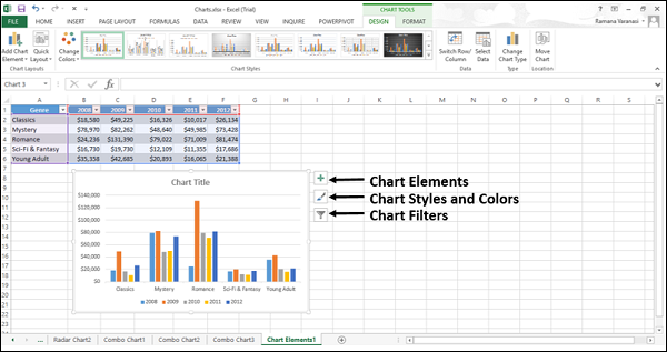
Chart Elements Button Excel

This menu is represented as a plus sign.
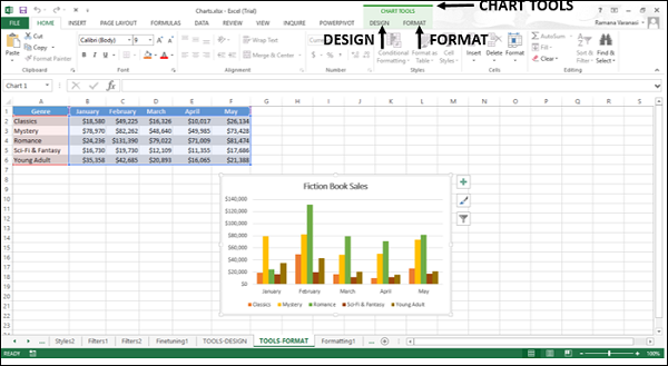
Chart elements button excel. Some chart elements such as a series legend or data label consist of multiple items. When you tick a checkbox Excel will add that chart element with default setting on the chart. Step 1 When you click on a chart CHART TOOLS comprising of DESIGN and FORMAT tabs appear on the Ribbon.
Right-click on the pie and select Add Data Labels. Press with mouse on Chart title. Chart Elements Not Showing Up i am using Excel 2016 and am having difficult with the on-object chart customization buttons.
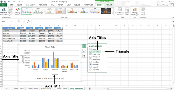
Locate the Chart section and deselect either or both of the check boxes labeled Show Chart Element Names On Hover or Show Data Point Values On Hover. Excel Charts Design Tools. Or activate the Design tab of the ribbon under Chart Tools and click Chart Element Axis Titles then select the option you want.
If you want to add only one of the two you can add both then click on the one you dont want and press Delete. I looked and my excel is version 1515. No drop down comes up.
Step 2 Click the DESIGN tab on the Ribbon. Where is the chart elements button in Excel. On the Format tab in the Current Selection group click the arrow next to the Chart Elements box and then select the.
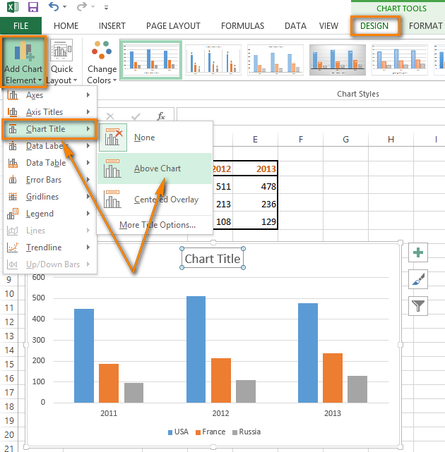
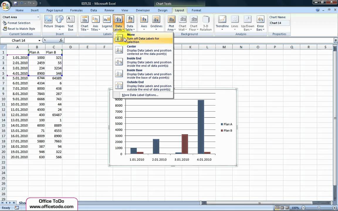
This feature also supports Live Preview so even if you dont know what each element is you can easily preview what the chart would look like with any. Click anywhere in the chart. Step 1 Click Add Chart Element.
One of the Form Control tools the Option Buttons will also help make the chart interactive. I have an office 365 subscription so I thought I would have the most up to date version. The chart now shows that the chart title selected.
2 Click the second button from it. 22 How to delete the chart title. We can still use them.
Press with left mouse button on Add Chart Elements button. Adding and removing any chart element is as easy as a single click. Press Delete key on your keyboard.
Now it instantly creates the 3-D pie chart for you. Since Excel 2013 Mircosoft provided a fly-out menu with Excel Charts that lets us add and remove chart elements quickly. Ive attached a screen shot.
When I get to this point Im unable to click on the Add Chart Element button. Im simply opening Excel and filling in a few cells to make a scatter plot. The Format pane appears with options that are tailored for the selected chart element.
Press with mouse on the chart title with left mouse button. This displays the Chart Tools adding the Design Layout and Format tabs. 3 Under style option click on the required style.
1 Click on the chart and in the right top corner three buttons appear at the edge of the chart. My chart isnt shared. Excel tutorial on how to add Option Buttons to filter a chart.
This will add all the values we are showing on the slices of the pie. Step 1 On the Ribbon click Quick Layout. Press with mouse on Above Chart.
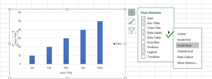
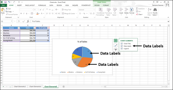
Clicking on the Chart Elements button will launch a simple and easy-to-use checklist of all the different elements you can add to your chart. Select the data to go to Insert click on PIE and select 3-D pie chart. 4 Under color option choose a color from the different color scheme.
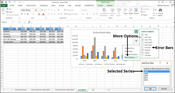
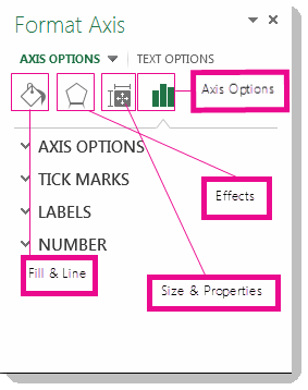
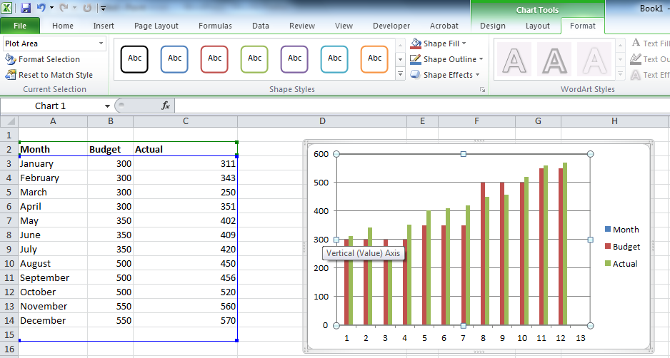
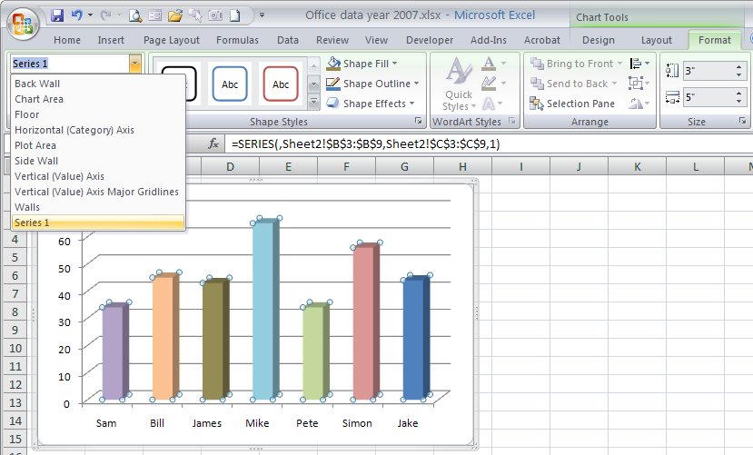
Select the chart element for example data series axes or titles right-click it and click Format. They do not show up when I select my graph. As soon as you click on this sign all the chart elements will be shown with checkboxes before them.
Clicking the small icons at the top of the pane moves you to other parts of the pane with more options.