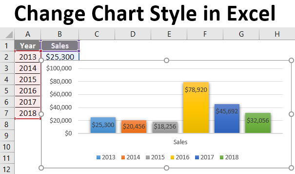
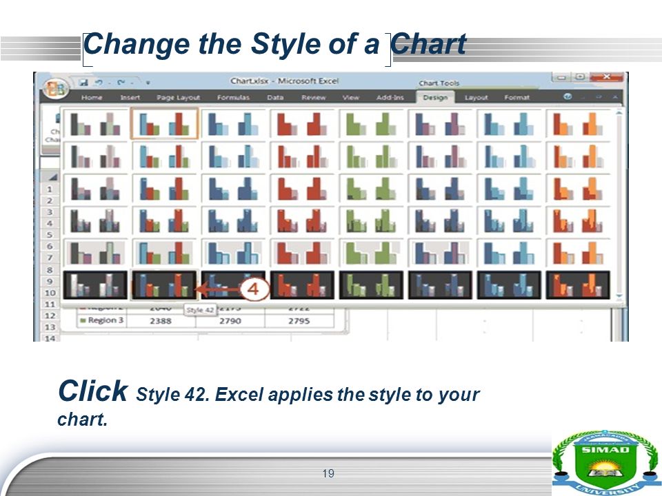
Change The Chart Style To Style 42
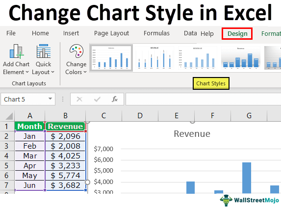
You can change the style of an existing chart for a different look.
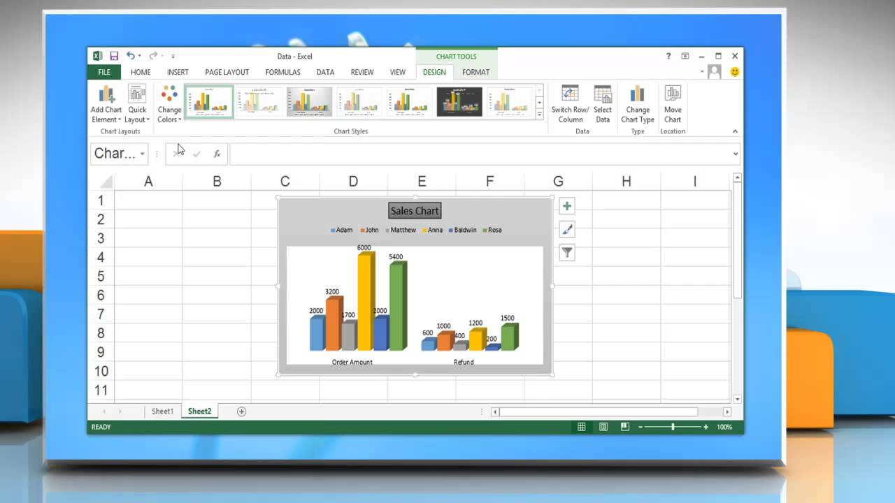
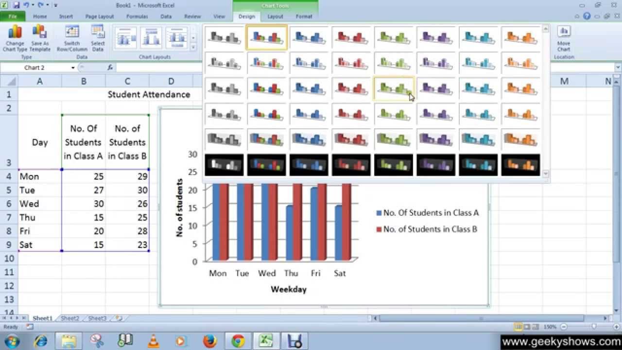
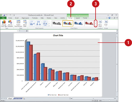
Change the chart style to style 42. Step 2 Click the Chart Styles icon. The Design tab will appear. All in One Excel VBA Bundle 35 Courses with.
Click Style 7 to change the charts style. Even better these styles are influenced by Office Themes. Watch what happens to your chart when you select a style.
To change the chart style. Lets see how to format the charts once inserted. The following code example adds a 3-D clustered column chart to Sheet1 and sets its style to style 4.
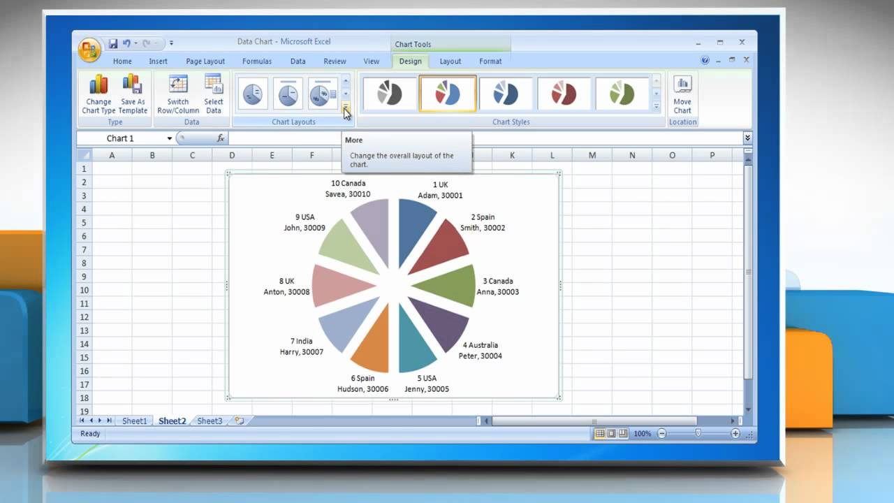
Clicking the More drop-down arrow. There one will see all the options and can easily change from Style to Style 42. You can use STYLE to fine tune the look and style of your chart.
Go to options and then fonts and styles. Learn how to insert a. Just a couple of clicks can make your charts look distinctive.
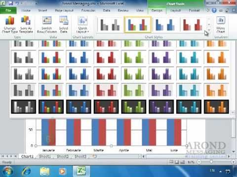
Select a style from 2D charts. Work your way through the Styles and click on each one in turn. Tornado Chart in Excel.
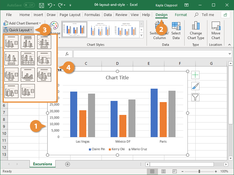
Now we will see how to change the styles. On the Design tab in the Chart Layouts group click Quick Layouts and then click the first chart layout Layout 1. Step 3 Choose the style option you want.
On the Format tab in the Current Selection group click the arrow in the Chart Elements box and then click the chart element for which you want to change the formatting style. Click The More Arrow In The Chart Styles Section. An integer from 1 through 48 that represents the style of the chart.
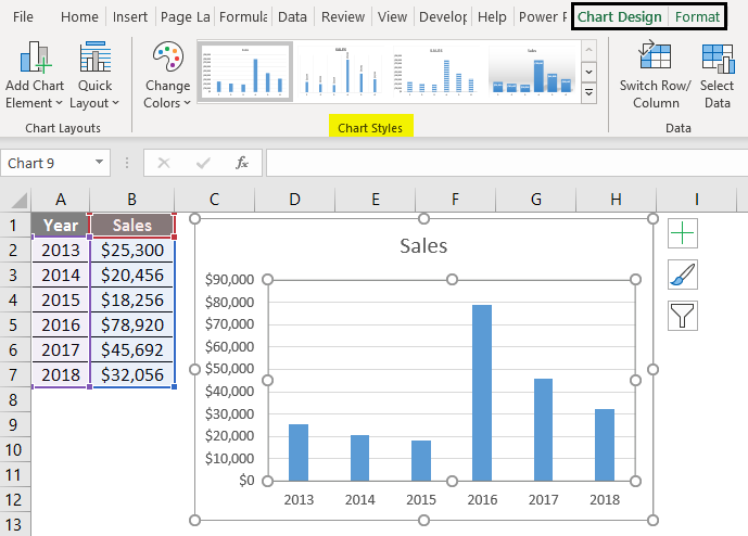
Table Styles in Excel. From the Design tab click the More drop-down arrow in the Chart Styles group. Point to any of the options to see the preview of your chart with the currently selected style.
Add Filter in Excel. When you select your chart you can observe the Style are available in the design Tab of the Excel ribbon. Bar charts look like different bars with both vertical and horizontal styles available.
Please enable it to continue. The chart will appear in the selected style. Click the chart element that you want to change or do the following to select it from a list of chart elements.
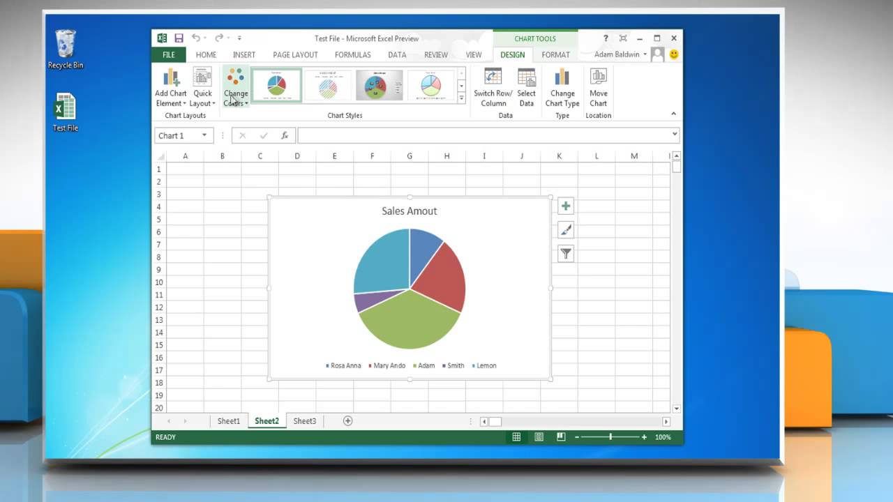
Were sorry but dummies doesnt work properly without JavaScript enabled. Different style options will be displayed. We have different options to change the color and texture of the inserted bars.
Windows macOS For most 2-D charts you can change the chart type of the whole chart to give the chart a different look or you can select a different chart type for any single data series which turns the chart into a combination chart. To the right of the chart click the Chart Styles action button to display the Chart Styles gallery. This has been a guide to Change Chart Style in Excel.
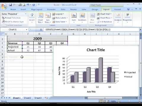
Click The Design Tab. Click The Quarterly Sales Checkbox. Next the code specifies the colors of the chart walls and floor.
And heres the Styles in Excel 2013 to 2016. Step 1 Click STYLE. On the Presentation worksheet select the chart.
Change The Chart Style To Style 8 Click The Copy Button. How do you change the chart Style to Style 42 in Excel. This displays the Chart Tools adding the Design Layout and Format tabs.
Select the chart you want to modify. STYLE and COLOR will be displayed. To apply a Chart Style you first need to have a chart in your presentation.
If you are looking for the steps about how to change the layout or style of a chart in Microsoft Excel on a Windows 7-based PC Please follow the steps s. Click The Territory Checkbox. To see more styles click the arrows to the right of the Chart Styles panel.
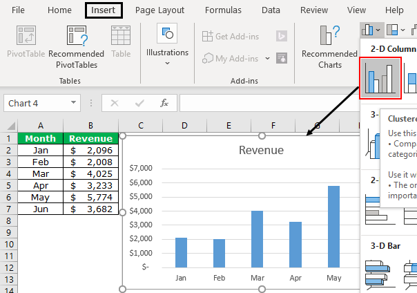
More styles in Excel 2013. Click The Insert Tab. Youll then see a drop down sheet of new styles Excel 2007.
It will instantly apply specified chart style. Each style comes with many color schemes and looks you can also tweak with applied chart style in order to make it look like you want. The example then creates a range of arbitrary data and sets it as the chart source data.
Following are the Styles in Design tab Excel 2013 Ribbon Menu. You may also look at these useful articles on excel Animation Chart in Excel. To view more styles you can click on the scroll bar at right side of the styles.
For bubble charts and all 3-D charts you can only change the chart type. Select the desired style from the menu that appears. Click on any chart style and your chart will change.
To apply chart styles select the chart and head over to Design tab under Chart Styles gallery select a desired one to apply. These Chart Styles include predefined combinations of various chart elements and include effects and layouts that can change their appearance. Here we discuss step by step how to change the chart style in excel along with examples a downloadable excel template.
Click The Paste Drop-down Menu Then Click Values. Step 2 Scroll down the options. Practical Learning Applying Chart Styles in Excel.