Pie Chart In Excel

Excel pie charts are useful to display fractions of a whole by splitting a circle into sections. Steps to Create a Pie Chart Select the Insert tab in the toolbar at the top of the screen. Create a pie of pie or bar of pie chart in Excel.

who should i vote for flow chart ngk spark plug chart stanford football depth chart 2014 steak cooking temp chart bristol motor speedway seating chart accounting chart of accounts historical stock market returns by year chart lularoe classic t size chart

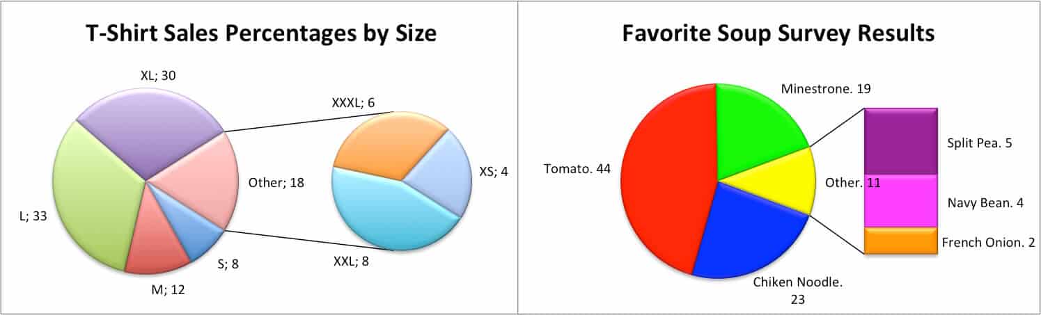
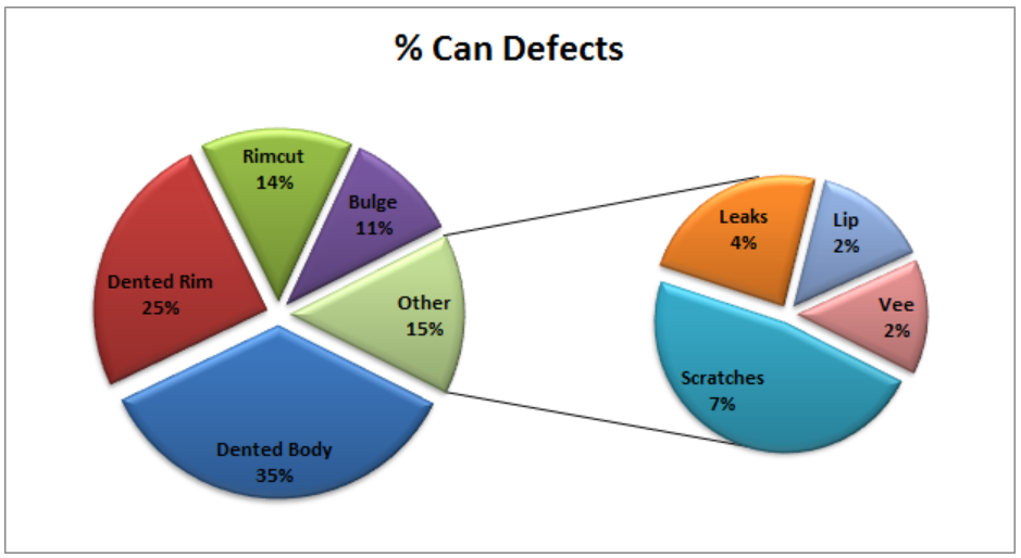
Creating Pie of Pie Chart in Excel.

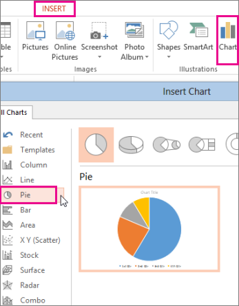
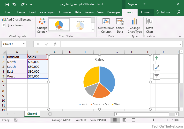
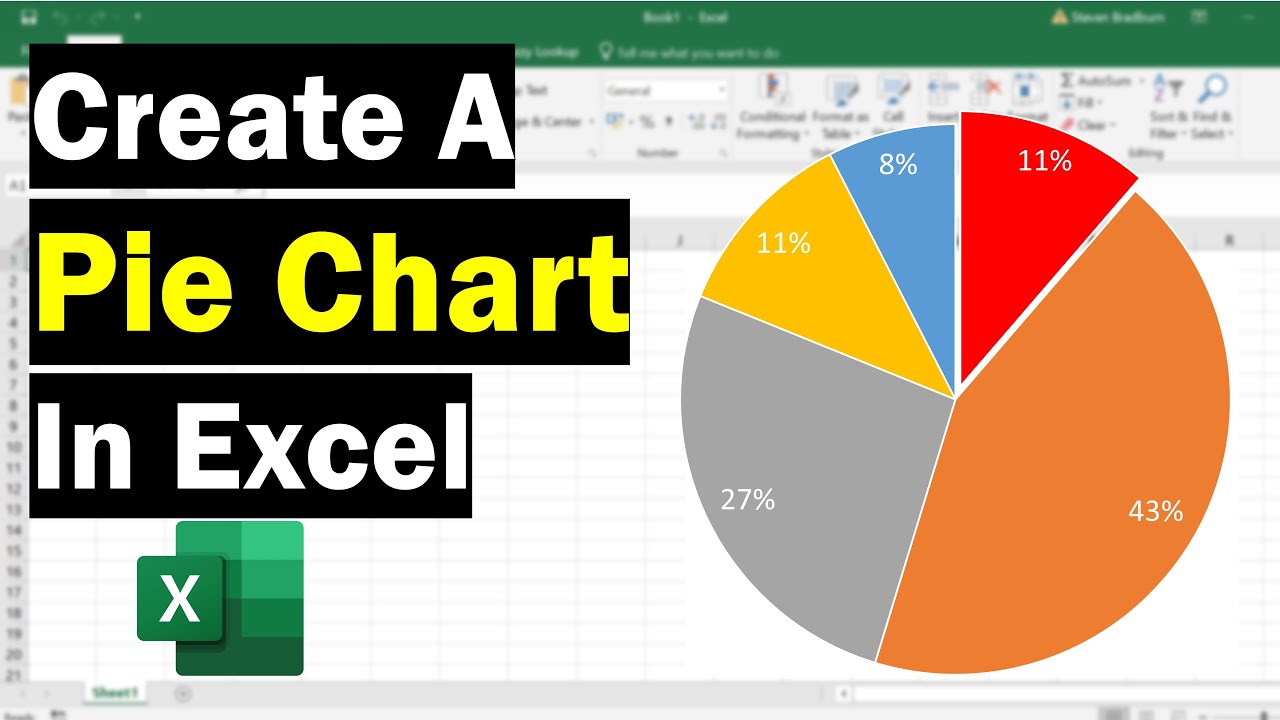
Pie chart in excel. In Excel Click on the Insert tab. Click on the drop-down menu of the pie chart from the list of the charts. Stick around to learn all about how to quickly build and customize pie charts.

Once you have all your data in place follow these steps to create a pie chart. Pie charts are used to display the contribution of each. Click on the Insert tab.

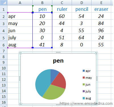
Now in the charts group you need to click on the Insert Pie or Doughnut Chart option. The pie chart is commonly used and for good reason. Add a Pie Chart.

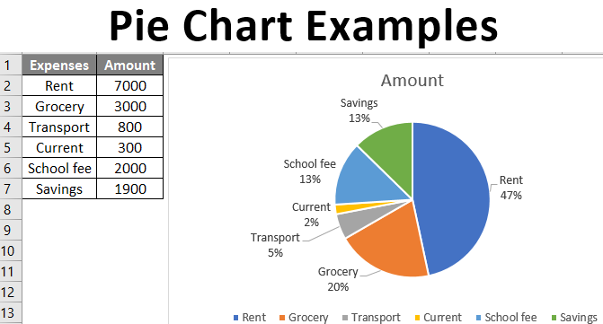
Select the entire dataset of the table you just made D4E6. Heres how we do it. To create a pie chart in Excel 2016 add your data set to a worksheet and highlight it.

Now select Pie of Pie from that list. Click on the pie icon that is within the 2-D pie icons. Click on the Pie icon within 2-D Pie icons.

The Pie Chart obtained for. How to create a pie chart. Below is the Sales Data were taken as reference for creating Pie of Pie Chart.

Switch to the Insert tab. Once you have all the necessary data ordered its high time to bring it to life with the help of a pie chart. Pie charts can be moved around within the Excel sheet.

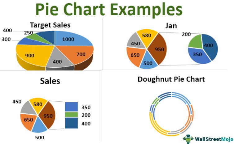
Click on the Pie button in the Charts group and then select a chart from the drop down menu. Choose Insert Pie or Doughnut Chart. A pie of pie or bar of pie chart it can separate the tiny slices from the main pie chart and display them in an additional pie or stacked bar chart as shown in the following screenshot so you can see the smaller slices more visible or easier.

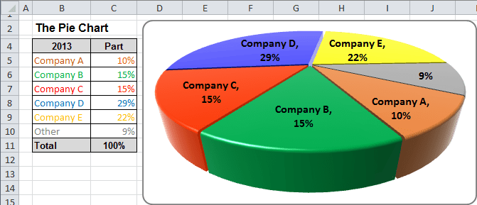
Its one of the best Excel charts you can use. Click on the pie icon that is within the 2-D pie icons. If we choose to make a 3D pie chart it will look like this.

Click Insert tab Pie button then choose from the selection of pie chart types. Excel Pie Chart Template Free Download. Creating a Pie Chart in Excel.

In the Charts group click on the Insert Pie or Doughnut Chart icon. Pick the chart you want we chose the simplest. Click the Insert tab.

It presents data efficiently shows both values and proportions and is very easy to read. Lets see how to create Pie of Pie chart in Excel. Now you will see the completed pie chart.

On top of that its easy to make. Select the chart type you want to use and the chosen chart will appear on the worksheet with the data you selected. Select the whole dataset.

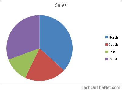
A pie chart also known as a circle chart is a circular graph where each slice illustrates the relative size of each element in a data set. Select the entire dataset. Just like any chart we can easily create a pie chart in Excel version 2013 2010 or lower.

The Fastest Way to Create a Pie Chart in Excel. First we select the data we want to graph. Go to the Insert tab and click the Pie Chart drop-down arrow.

In this example we have selected the first pie chart called Pie in the 2-D Pie section. Pie Exploded Pie Pie of pie Bar of pie or 3D pie chart. Then click the Insert tab and click the dropdown menu next to the image of a pie chart.